Last Layer KV Cache is All You Need
TL;DR — LastKV lets every layer read one shared last-layer history. It reduces long-term KV storage toward 1/L of a standard L-layer Transformer and feeds deep past representations back into future computation. Recurrence happens across chunks, while tokens within each chunk are processed in parallel.
Despite substantially compressing history, LastKV matches or outperforms standard Transformers across language modeling, state tracking, novel view synthesis, and video generation.
One history for every layer
Transformers store separate key–value (KV) states at every layer, causing memory to scale with network depth while preventing deep representations of the past from informing shallower future layers. In LastKV, all layers instead share the last-layer KV states of completed context. This reduces long-term KV storage by approximately the number of layers and creates recurrence across both time and depth.
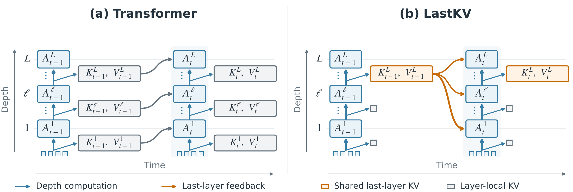
Share the deepest states
Every layer attends to the last-layer KV of completed chunks alongside its own current-chunk KV. Past tokens remain directly accessible through attention.
Keep chunks parallel
Tokens within a chunk use ordinary causal attention. Once the chunk completes, its last-layer KV is appended to the shared history for subsequent chunks.
Blend recent context
Learned per-head gates combine layer-local and last-layer KV for the immediately preceding chunk, smoothing the transition at chunk boundaries.
With L layers, T tokens, and C tokens per chunk, the persistent KV ratio relative to a standard Transformer is (T + (L − 1)C) / (LT), which approaches 1/L as the number of chunks grows.
The limit assumes equal KV widths and deduplicated storage. It counts persistent KV entries; temporary buffers and training activations are excluded. Dense attention remains quadratic.
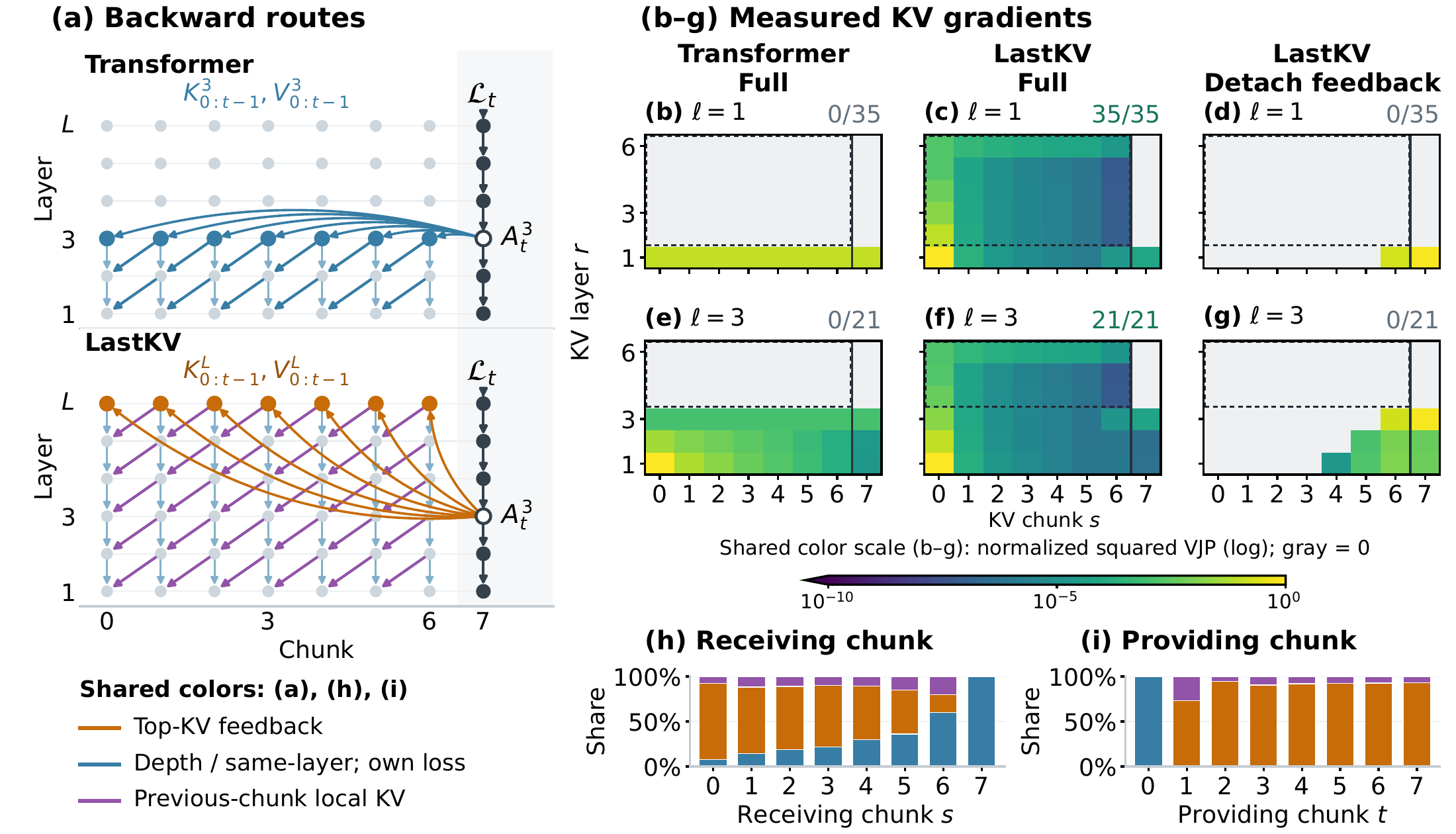
Recurrence and gradient flow
Long-context language modeling
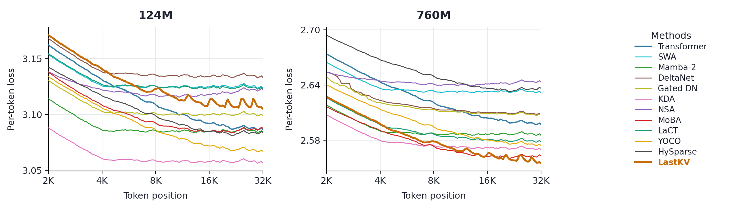
We pretrain 124M and 760M models at 32K context. Tail loss measures the 30K+ portion of the sequence; RULER accuracy averages evaluations at 4K, 8K, 16K, and 32K. LastKV improves average retrieval at both scales.
| 124M | 760M | |||
|---|---|---|---|---|
| Model | Tail loss ↓ | RULER ↑ | Tail loss ↓ | RULER ↑ |
| Transformer | 3.0869 | 16.52 | 2.598 | 34.2 |
| Mamba-2 | 3.085 | 13.0 | 2.586 | 23.5 |
| Kimi Delta Attention | 3.057 | 12.1 | 2.571 | 22.8 |
| MoBA | 3.0872 | 14.70 | 2.563 | 34.2 |
| LaCT | 3.123 | 8.5 | 2.579 | 23.2 |
| YOCO | 3.0672 | 15.14 | 2.575 | 26.4 |
| HySparse | 3.0835 | 18.74 | 2.636 | 30.2 |
| LastKV | 3.1067 | 20.05 | 2.556 | 34.3 |
Selected baselines; RULER in %. Bold marks the best value in each column. At 124M, LastKV’s tail loss is higher than Transformer; at 760M, its tail loss is lower and the average retrieval advantage is small at the displayed precision. The paper reports all baselines and per-length RULER results.
State tracking and memory retention
LastKV is best or tied-best on five of the seven synthetic task families in the full comparison. The paired results below report token accuracy at 2K context.
| Task | Transformer | LastKV |
|---|---|---|
| Fixed finite-state automaton | 40.7 | 43.2 |
| Mode switch | 78.8 | 92.6 |
| Generalized modular sum | 11.4 | 21.3 |
| Group word | 25.3 | 27.6 |
| Permutation composition | 57.7 | 59.8 |
| Multi-query associative recall | 68.4 | 100.0 |
| Selective copy | 99.9 | 100.0 |
Token accuracy (%), higher is better. Bold marks the best value among all methods in the paper’s full comparison.
Novel view synthesis
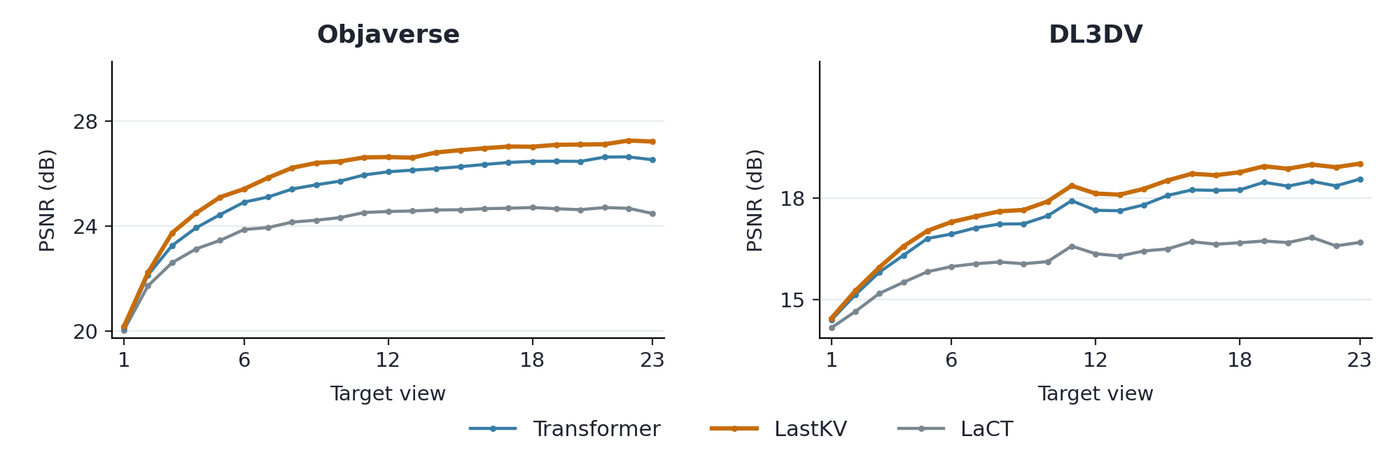
Sharing last-layer KV improves reconstruction PSNR on both evaluated datasets.
| Model | Objaverse PSNR ↑ | DL3DV PSNR ↑ |
|---|---|---|
| Transformer | 25.36 | 17.41 |
| DeltaNet | 23.94 | 15.82 |
| Gated DeltaNet | 24.32 | 16.05 |
| LaCT | 23.99 | 16.14 |
| LastKV | 25.94† | 17.80 |
PSNR in dB. Bold marks the best value in each column. † The Objaverse LastKV result uses logged in-training evaluation with random view draws. Other NVS results use fixed-view full-test evaluation.
Loss and reconstruction curves
Autoregressive video generation
LastKV improves VBench total scores at both 1.3B and 14B after teacher-forced fine-tuning.
| Model | Quality ↑ | Semantic ↑ | Total ↑ |
|---|---|---|---|
| Transformer 1.3B | 83.1 | 76.5 | 81.8 |
| LastKV 1.3B | 83.5 | 78.0 | 82.4 |
| Transformer 14B | 82.2 | 72.7 | 80.3 |
| LastKV 14B | 83.0 | 76.4 | 81.6 |
VBench scores (%), from 4,730 generated videos: 946 prompts × five samples. Bold marks the better value at each size. The paper provides the full VBench breakdown and user-study protocol.
Selected 14B examples
Five selected comparisons highlighting LastKV’s prompt adherence and visual coherence. Each pair uses the same prompt.
Loading examples…
Prompt:
Less cache, with measured training costs
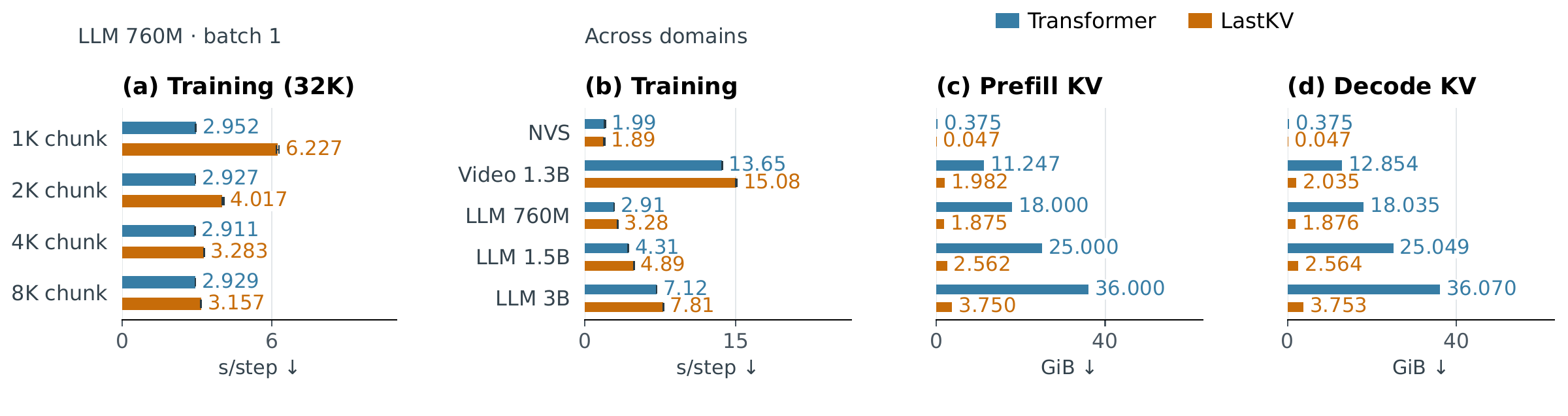
LastKV substantially reduces physical self-attention KV allocation after prefill and cached decoding. The comparisons use matched workloads, precision, and A100-SXM4-80GB hardware. LLMs train at 32K and use a 128K inference prefix with 4K chunks.
| Train (s/step) ↓ | Prefill KV (GiB) ↓ | Decode KV (GiB) ↓ | ||||
|---|---|---|---|---|---|---|
| Workload | Transformer | LastKV | Transformer | LastKV | Transformer | LastKV |
| NVS | 1.99 | 1.89 | 0.375 | 0.047 | 0.375 | 0.047 |
| Video 1.3B | 13.65 | 15.08 | 11.247 | 1.982 | 12.854 | 2.035 |
| LLM 760M | 2.91 | 3.28 | 18.000 | 1.875 | 18.035 | 1.876 |
| LLM 1.5B | 4.31 | 4.89 | 25.000 | 2.562 | 25.049 | 2.564 |
| LLM 3B | 7.12 | 7.81 | 36.000 | 3.750 | 36.070 | 3.753 |
Absolute training time and physical self-attention KV allocation; bold marks the lower value in each pair. LLM decode KV follows 128 additional tokens. The 1.5B and 3B training fixtures use matched random initialization to measure runtime.
What the results establish
Sharing the last-layer history reduces persistent KV storage toward 1/L while LastKV matches or outperforms standard Transformers across the four task domains in the reported settings. The gains are not uniform: at 124M, LastKV’s long-context tail loss is higher than Transformer’s, and at 760M its average retrieval advantage is small at the displayed precision. The Objaverse LastKV result uses in-training evaluation with random view draws; the other NVS results use the fixed-view protocol.
Physical KV savings are not total GPU-memory savings, and training time increases in the reported LLM and video configurations. Dense attention remains quadratic, and broader gradient connectivity alone does not establish better optimization.
Citation
@misc{cai2026lastkv,
  title  = {Last Layer {KV} Cache is All You Need},
  author = {Cai, Zefan and Bi, Sai and Zhang, Lin and Hong, Yicong and
            Zhu, Yuchen and Li, Lu and Zhao, Haozhe and Jiang, Hanwen and
            Hu, Qinzhe and Huang, Zeyi and Lin, Shawn and Luo, Cheng and
            Ge, Chongjian and Jian, Jinlin and Zhu, Ruijie and Huang, Xun and Gu, Jiuxiang and
            Hu, Junjie and Tan, Hao},
  year   = {2026},
  note   = {Preprint},
  url    = {https://zefan-cai.github.io/LastKV.github.io/}
}